Sound Recognition
Overview
Machine Learning techniques are often used in identifying trends and categorizing data. These trends are then leveraged to inform strategic decisions. There are several applications of this in the field of finance, economic research, and software development. However, one field that hasn’t been explored as much is audio. This project attempts to understand the capabilities of machine learning techniques in detecting sources of audio files. Leveraging Python's diverse libraries, the project focuses on extracting distinctive audio features from voice samples of different individuals. The primary goal was to train a model to recognize voices based on these features and classify a given audio sample to its correct source.
Libraries Utilized

Librosa
A Python package dedicated to the analysis of audio and music. It offers utilities to extract information from audio signals.
Pandas
Utilized for feature extraction from the dataset. The intuitive data structures provided by pandas helped in the organization, cleaning, and manipulation of audio data.

TensorFlow
While TensorFlow is capable of building complex neural network architectures, for this project, it was employed to visualize the neural network's structure, aiding in understanding and debugging.
Matplotlib
It played a vital role in this project to visually represent the relationship between various extracted audio features. By plotting these relationships, insights could be drawn about the nature and characteristics of the audio data.
Scikit-learn
The ‘MLPClassifier’ module was leveraged to implement a neural network model. This classifier allowed for the customization of the network structure and training parameters to fit our dataset.
Numpy
It enabled the transformation and reduction of these multi-dimensional datasets, preparing them for input into the neural network model.
Data
Dataset: The dataset consisted of 25 unique audio files from different individuals. This collection of varied voice samples served as the foundation for the audio classification model.
Key Characteristics:
Variability: Every voice is unique which brought in diversity in terms of voice patterns, pitches, and timbres to the data.
Audio Length: The durations of these files varied, reflecting natural variations in spoken content.
Sampling Rate: While original sampling rates might have differed, they were standardized during the preprocessing phase.
Languages & Accents: The dataset wasn't focused on languages or accents, but the potential presence of different languages or accents added another layer of complexity.
Data Preprocessing
Data preprocessing was a fundamental part of this project. It ensures that the raw audio data is transformed and conditioned to be suitable for our neural network model. Given the complexity of audio signals, a rigorous preprocessing pipeline was essential.
Here's how it was done:
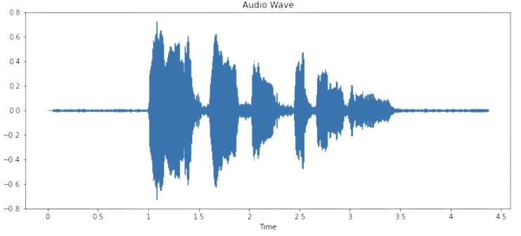
1. Audio Feature Extraction with Librosa: Mel-frequency cepstral coefficients (MFCCs) of audio clips were extracted using Librosa. MFCCs provided a compact representation of the audio, capturing the audio's timbral texture. Each audio file was represented by a fixed-size vector of MFCCs, standardizing the input shape for the neural network.
2. Dimensionality Reduction with Numpy: Audio features, especially when processed, can yield multi-dimensional data that is difficult to perform any sort of operation on. Using Numpy, these multi-dimensional arrays were transformed into manageable sizes. This step was crucial to ensure that the neural network received data in a consistent and computationally efficient format.
3. Normalization of sampling rate: To ensure that the neural network model trained effectively, it was essential to scale the features such as sampling rate so they had a consistent representation. This prevented certain features from disproportionately influencing the model due to their larger numeric range.
4. Data Privacy Considerations: Ensuring data privacy was paramount. All audio files were anonymized, stripping away any personal identifiers.
5. Data Splitting: Once the audio data was preprocessed, it was divided into training and testing sets. This ensured that there was a separate dataset to evaluate the model's performance post-training.
Key Features Extracted
Zero Crossing Rate: This feature calculates the rate at which the audio signal changes its sign. It measures the number of times a sound waveform crosses a reference amplitude (usually zero). A high zero crossing rate might indicate a noisier signal or a more complex harmonic structure. It's an essential metric for distinguishing between percussive sounds and harmonic sounds which can be especially relevant when dealing with voice data.
Spectral Frequency: It represents how various frequencies contribute to the sound signal by analyzing the distribution of amplitude against its frequency. This feature can highlight the dominant frequencies present in the voice data and gives insight into the vocal range and any unusual frequency peaks which might represent specific vocal characteristics or artifacts.
Spectral Flatness: This quantifies how noise-like a sound is compared to being tone-like. A perfectly tonal signal (single frequency) has a spectral flatness close to 0, whereas a perfectly noise-like signal has a spectral flatness close to 1. For voice data, spectral flatness can indicate the clarity of a sound sample or the presence of background noise.
Mel-Frequency Cepstrum (MFC): MFC is a representation of the short-term power spectrum of sound. It's based on the known variation of the human ear's critical bandwidths with frequency, making it especially suited for human voice processing. It can provide a compact representation of an audio clip in the frequency domain. For voice data, MFC coefficients (MFCCs) can capture the essential characteristics of voice timbre, thus enabling it to differentiate between different people effectively.
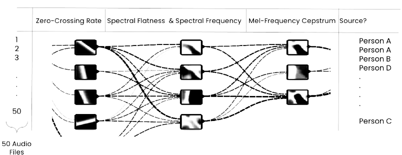
Process of analyzing features to decipher source of audio file
Machine Learning Model
Algorithm Used: Neural Networks (MLPClassifier from sklearn).
Accuracy: ~90%
Configuration:
Hidden Layers: Two hidden layers with 6 and 7 neurons respectively.
Activation Function: Tanh (Hyperbolic Tangent).
Solver: Stochastic Gradient Descent (SGD).
Learning Rate: Initialized at 0.1 and set to adaptive mode, adjusting as the model converges.
Max Iterations: 500 (defines the number of times the model would train on the dataset).